When it comes to deployment observability there are multiple, comprehensive solutions that can handle almost any system of scale you throw at them. I said almost, because there are certain stories that do not require setting up a central monitoring server with satellite agents to collect and enrich data.
For an example, consider a scenario where you’re troubleshooting a certain single process for a particular period of time. You want to collect the approximate CPU usage, approximate memory usage, light weight process (aka thread) count, and the TCP connection count. You want these stats collected during the time period you’re conducting load test against the process.
There are a list of well established tools that could provide the results we need. However, with sophisticated functionality comes complex setup instructions. Even if you skip a system with agent based monitoring, you’ll still be yum install ing, apt-get ting, or make install ing stuff. Sometimes the window is too narrow for these to be done, so much that by the time you’re setup, the issue has been resolved in some mysterious way that you start believing in miracles again.
After a little bit of Googling, I wanted to write something myself (living the dream!). I wanted to use as minimum bootstrapping as possible to collect a reasonably accurate set of metrics for a brief period of time. I wanted the collected stats to be human readable as well as quickly converted to a visualization.
I wanted something dot slashable instead of setting up an Icinga2 setup.
Bashfu Again!
I have to admit, Bash is kind of the proverbial hammer for almost every problem of mine. It’s easy to become so. Quickly written, quickly tested, and quickly deployed, Bash scripts are one of the most versatile tools I’ve come across.
So to come back to the problem again, I wanted to collect metrics for a single process, for a controlled period of time, and output (somewhat) both human and machine readable numbers.
Comma Separated Values (CSV) is the obvious easy choice here, though there could be more sophisticated options. A CSV file
- can be loaded to a spreadsheet application which then can visualize the data easily
- can be easily written by a script
- can be easily read to understand the values
Now it’s just a matter of collecting the information.
CPU and Memory Usage
To keep to the principle of using minimal bootstrapping, I opted to use the top tool to collect CPU and Memory usage.
cpu_mem_usage=$(top -b -n 1 | grep -w -E "^ *$pid" | awk '{print $9 "," $10}')
top -b -n 1 — top command run in the batch mode once
grep -w -E "^ *$pid" — look for the entry for the process ID we are looking for
awk '{print $9 "," $10}' — get the CPU and memory usage values
Thread Count
Another everyday tool to the rescue.
tcount=$(ps -o nlwp h $pid | tr -d ' ')
ps -o nlwp h $pid — print the number of light weight processes (threads) for the particular process (without the header — h)
tr -d ' ' — remove any spaces
TCP Connection Count
I wanted to count the number of outgoing TCP connections the process made during the load testing (we wanted to see if setting TCP keep_alive settings were making any difference).
tcp_cons=$(lsof -i -a -p $pid -w | tail -n +2 | wc -l)
lsof -i -a -p $pid -w — print all the Internet (ipv4 and ipv6) connections for the process suppressing any errors
tail -n +2 — Remove the header line from selection
wc -l — Count the number of lines
Of course, there are other ways to collect the same information. The accuracy of some of the metrics, like the CPU usage, can be argued about too.
This information is then written as a CSV entry into a file.
timestamp=$(date +"%b %d %H:%M:%S")
cpu_mem_usage=$(top -b -n 1 | grep -w -E "^ *$pid" | awk '{print $9 "," $10}')
tcp_cons=$(lsof -i -a -p $pid -w | tail -n +2 | wc -l)
tcount=$(ps -o nlwp h $pid | tr -d ' ')

echo "$timestamp,$cpu_mem_usage,$tcp_cons,$tcount" >> $csv_filename
Visualization
In terms of data collection, this is enough. However, we could go a bit further with minimal tools. For an example, let’s plot this data as graphs to get a better idea on spikes during the selected time period.
Plotting graphs is also a task with a lot of options in Bash. Out of these, gnuplot is the best tool to start with. It’s a well established tool (started out in 1986) with little complexity at its core.
We have to break our aim on using existing tools here though. Most systems do not have gnuplot packed in.
sudo apt install gnuplot
That should do for Ubuntu/Debian.
gnuplot can work with a variety of data files. To let it know that the input file is a CSV we can set the datafile separator .
set datafile separator ","
It also supports a number of output formats. In this story, we only need a graph output to an image file. We can set this information with the following. We are specifying the png output ( pngcairo is only available in certain systems but produce better looking anti-aliased lines), with image dimensions of 1024 x 800 .
set term pngcairo size 1024,800 noenhanced font "Helvetica,10"
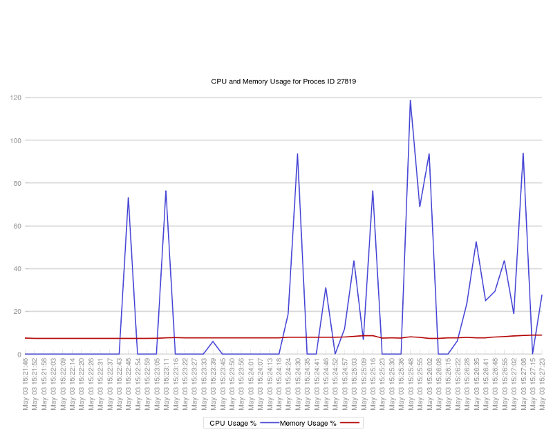
The first graph to plot is the CPU and memory usage.
set output "${dir_name}/cpu-mem-usage.png"
After setting the filename, the graph plotting is done, specifying the functions to perform on the data.
plot "$csv_filename" using 2:xticlabels(1) with lines smooth unique lw 2 lt rgb "#4848d6" t "CPU Usage %",\
       "$csv_filename" using 3:xticlabels(1) with lines smooth unique lw 2 lt rgb "#b40000" t "Memory Usage %"
$csv_filename — The data set to use
using 2:xticlabels(1) — Graph the second column using the first column as string labels on the X axis
with lines — Graph a line chart
smooth unique — Smoothen lines
lw 2 — Line width should be 2
lt rgb "#4848d6" — Define a line type with a color #4848d6
t "CPU Usage %" — Label of the chart
If we look at our Bash script line which writes to the CSV file, we can see that the second column contains the CPU metrics, while the first column contains the time stamp value.
We can plot the memory usage (third column) on the same graph.
"$csv_filename" using 3:xticlabels(1) with lines smooth unique lw 2 lt rgb "#b40000" t "Memory Usage %"
Likewise the other metrics can be plotted separately,
# TCP count
set output "${dir_name}/tcp-count.png"
set title "TCP Connections Count for Proces ID $pid"
plot "$csv_filename" using 4:xticlabels(1) with lines smooth unique lw 2 lt rgb "#ed8004" t "TCP Connection Count"

# Thread count
set output "${dir_name}/thread-count.png"
set title "Thread Count for Proces ID $pid"
plot "$csv_filename" using 5:xticlabels(1) with lines smooth unique lw 2 lt rgb "#48d65b" t "Thread Count"
or together.
set output "${dir_name}/all-metrices.png"
set title "All Metrics for Proces ID $pid"
plot "$csv_filename" using 2:xticlabels(1) with lines smooth unique lw 2 lt rgb "#4848d6" t "CPU Usage %",\
        "$csv_filename" using 3:xticlabels(1) with lines smooth unique lw 2 lt rgb "#b40000" t "Memory Usage %", \
        "$csv_filename" using 4:xticlabels(1) with lines smooth unique lw 2 lt rgb "#ed8004" t "TCP Connection Count", \
        "$csv_filename" using 5:xticlabels(1) with lines smooth unique lw 2 lt rgb "#48d65b" t "Thread Count"

Of course these are not the only directives given to gnuplot for these graphs to be generated. Everything from the position of the key, to the axis line colors can be configured to the detail.
# Set border color around the graph
set border ls 50 lt rgb "#939393"
gnuplot has a interactive shell where these commands can be given. However, this story requires a less involved approach. All the directives can be provided to gnuplot through heredoc, or <<- EOF notation.
gnuplog <<- EOF
set terminal
EOF
The above will display all the output types supported on the system. Similar to above, all the directives are fed to gnuplot to produce the graphs.
Conclusion
More an exercise than a comprehensive tool, I collected all the above into a single script to be executed. The source is on Github.
./process-metrics-collector.sh <PID>
The aim of the script is to be executed on a remote server. What it does is to cover a narrow set of requirements at the lower end of the monitoring spectrum. On the other side are the tools like AppDynamics, Icinga, and graphing tools like Graphite, and Grafana. This would cover the stories where we wouldn’t have the time or the resources to setup a comprehensive system, just to monitor a single process for a brief period of time.
Written on May 15, 2018 by chamila de alwis.
Originally published on Medium